Linear Models
This section describes multivariate regression analysis using a variety of methods. When the data at hand is fat-tailed or cannot be transformed to be normally distributed, then the assumptions for ordinary least squares regression are violated. In such cases, we can use robust regression and ols-t regression. In other scenarios perhaps we are dealing with issues of multicollinearity or variable proliferation, then we have Lasso and Ridge to choose from.
OLS Regression
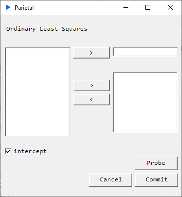
Description
Suppose we have the following system: $$ Y = X \beta $$
where
$$ X=\begin{bmatrix} x_{11} & x_{12} & \cdots & x_{1p}\\ x_{21} & x_{22} & \cdots & x_{2p}\\ \vdots & \vdots & \ddots & \vdots\\ x_{n1} & x_{n2} & \cdots & x_{np} \end{bmatrix} , \beta = \begin{bmatrix} \beta_1 \\ \beta_2 \\ \vdots \\ \beta_p \end{bmatrix} , Y = \begin{bmatrix} y_1 \\ y_2 \\ \vdots \\ y_n \end{bmatrix} $$
We solve the quadratic minimization problem given by: $$ \mathrm{\hat{\beta} = \underset{\beta}{\operatorname{arg\min}}\ F(\beta)} $$
where the objective function $ F $ is given by: $$ \mathrm{ F(\beta) = \sum_{i=1}^n \biggl| y_i - \sum_{j=1}^p X_{ij}\beta_j\biggr|^2 = | y - X \beta |^2 } $$
We obtain: $$ \mathrm{ \hat{\beta}= \left( X^{T} X \right)^{-1} X^{T} y } $$
Since matrix inversions are extremely high in time complexity, we use a QR decomposition to solve the system.
Returns
Main regression table and model metrics:
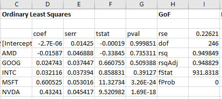
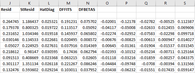
Goodness of fit measures and diagnostics:
- coef: coefficients
- serr: standard errors
- tstat: t-statistic
- pval: p-value
- rse: residual standard error
- dof: degrees of freedom
- rsq: r-squared
- rsqAdj: adjusted r-squared
- fStat: F-statistic
- fProb: p-value for model
- Resid: model residuals
- StResid: model standardized residuals
- HatDiag: hat diagonal
- DFFITS: studentized influence on predicted values
- DFBETAS: studentized influence on coefficients
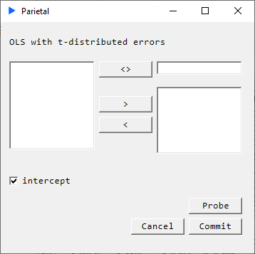
OLS with t-distributed errors
Description
We carry out a multivariate regression analysis but we assume that model errors are t-distributed.
$$ y = \mathrm{X} \boldsymbol{\beta} + \boldsymbol{\epsilon}, \boldsymbol{\epsilon} \sim t(\mu, \sigma, \nu) $$
An iterative method known as iteratively reweighted least squares (IRLS) is carried out until the estimates converge to an acceptable tolerance.
$$ \hat{\beta}^{(t+1)}=(X^{T}(W^{-1})^{t}X)^{-1}X^{T}(W^{-1})^{t}y $$
Returns
- coef: coefficients
- serr: standard errors
- tstat: t-statistic
- pval: p-value
- rse: residual standard error
- dof: degrees of freedom
- rsq: r-squared
- rsqAdj: adjusted r-squared
- fStat: F-statistic
- fProb: p-value for model
- Resid: model residuals
- StResid: model standardized residuals
Robust Regression
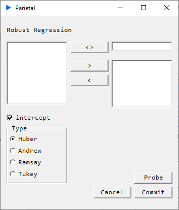
Description
The purpose of robust regression methods is to dampen the influence of outliers in data by specifying a weight function. A number of these weight functions have been proposed. We implement four of these:
- Huber
- Andrew
- Ramsay
- Tukey
An iterative method known as iteratively reweighted least squares (IRLS) is carried out until the estimates converge to an acceptable tolerance.
$$ \mathrm{\hat{\beta}^{t+1}=(X^{\textrm{T}}(W^{-1})^{t}X)^{-1}X^{T}(W^{-1})^{t}y} $$
where
$$ \mathrm{w_{i}^{t}= \begin{cases}\dfrac{\psi((y_{i}-x_{i}^{t}\beta^{t})/\hat{\tau}^{t})}{(y_{i} x_{i}^{t}\beta^{t})/\hat{\tau}^{t}} & {if (y_{i} \neq x_{i}^{\textrm{T}}\beta^{t})} \\ 1 & {if (y_{i}=x_{i}^{\textrm{T}}\beta^{t})} \end{cases}} $$
Returns
- coef: coefficients
- serr: standard errors
- tstat: t-statistic
- pval: p-value
- rse: residual standard error
- dof: degrees of freedom
- rsq: r-squared
- rsqAdj: adjusted r-squared
- fStat: F-statistic
- fProb: p-value for model
- Resid: model residuals
- StResid: model standardized residuals
Ridge Regression and CV
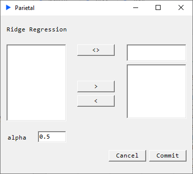
Description
Ridge regression is a form of penalized regression. The parameter that controls this penalty is $\alpha$ which can range from 0 (no penalty) to 1. The penalty prevents against a variable having an outsized coefficient compared to others.
$$ \hat{\beta}_{ridge} = (X^T X + \lambda I_p)^{-1} X^T Y $$
We solve for coefficients that minimize:
$$ \sum_{i=1}^n (y_i - \sum_{j=1}^p x_{ij}\beta_j)^2 + \lambda \sum_{j=1}^p \beta_j^2 $$
Returns
- coefficients
- MSE
- predicted values
Cross Validation Returns
- best $\alpha$
- best model MSE
- coefficients
- predicted values
- $\alpha$ path
- regularization path
- MSE grid
Lasso Regression and CV
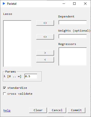
Elastic Net combines $L_{1}$ and $L_{2}$ penalties. The two parameters that control this penalty are $\lambda \in [0, \infty)$ and $\alpha \in [0, 1]$.
$\alpha$ balances Ridge and LASSO penalties with $\alpha = 1$ being LASSO. We use coordinate descent for the updates.
$$ \min_{(\beta_0, \beta) \in \mathbb{R}^{p+1}}\frac{1}{2N} \sum_{i=1}^N (y_i -\beta_0-x_i^T \beta)^2+\lambda \left[ (1-\alpha)||\beta||_2^2/2 + \alpha||\beta||_1\right], $$
where $ \lambda \geq 0 $ is known as the complexity parameter and $ \alpha \in [0, 1]\ $ is the ridge parameter.
If the cross validation option is checked, a 10-fold cross validation is performed. The $\lambda$ path used is generated using the method described by Hastie-Tibshirani [1].
Returns
- $\alpha$
- $\lambda$
- MSE
- coefficients
- predicted values
Cross Validation Returns
- $\alpha = 1$
- best model $\lambda$
- best model MSE
- coefficients
- predicted values
- $\lambda$ path
- regularization path
- MSE grid
[1] Regularization Paths for Generalized Linear Models via Coordinate Descent (Journal of Statistical Software - Jan 2010)
Least Absolute Deviation Regression
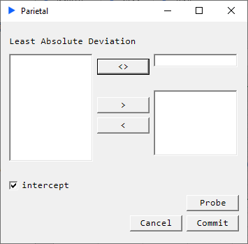
Description
Where OLS regression seeks to minimize the L2 norm, least absolute deviation (LAD) regression seeks to minimize the L1 norm $ S = \sum_{i=1}^n |y_i - f(x_i)| $ . We use iteratively weighted least squares (IRLS) to solve this problem. LAD is more resistant to outliers than OLS and is therefore typically considered a form of robust regression.
Returns
- coef: coefficients
- serr: standard errors
- tstat: t-statistic
- pval: p-value
- rse: residual standard error
- dof: degrees of freedom
- rsq: r-squared
- rsqAdj: adjusted r-squared
- fStat: F-statistic
- fProb: p-value for model
- Resid: model residuals
- StResid: model standardized residuals