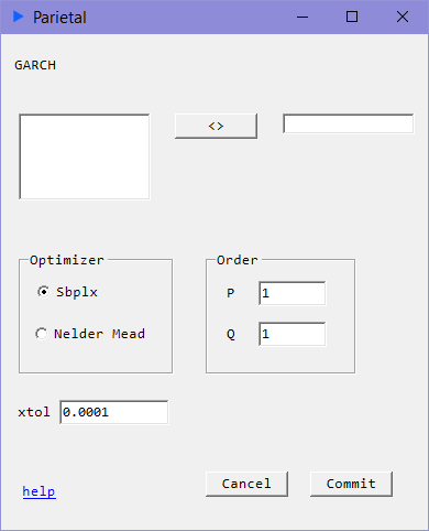
GARCH
Time Series Volatility

Description
Consider the following.
- Autocorrelation in squared returns
- Volatility clustering
- Conditional Normality i.e. $ f(y | y_{t-1}) \sim N(0, \alpha_{0} + \alpha_{1} y^{2}_{t-1}) $
The following relation would seek to model the above:
$$ \sigma_{t}^{2} = \alpha_{0} + \sum_{i=1}^{q}\alpha_{i}u_{t-i}^{2} + \sum_{i=1}^{p}\beta_{i}\sigma_{t-i}^{2} $$
$ p $ specifies the GARCH parameter where $ p >= 0 $ and $ q $ specifies the ARCH parameter where $ q >= 1 $
GARCH(p, q) models attempt to capture volatility dynamics in time series. When $ p = 0 $, it is simply an ARCH(q) model. The key difference between the two is that GARCH captures long run volatility whereas ARCH models end their volatility capture at lag q.
We recommend using 100 * (log returns) as input series for numerical stability reasons.
This routine uses maximum likelihood estimation to fit the model.
GARCH models can sometimes be a bit troublesome to fit via MLE. The user is encouraged to try the MCMC methods for Garch(1, 1), Garch (2, 1) and Stochastic Volatilty models as an alternative.
Inputs
- xtol: tolerance for convergence test
- Optimizer: Sbplx, Nelder Mead
Returns
- coef: Coefficient estimates for $g$ for GARCH parameters and $a$ for ARCH parameters
- serr: Standard Errors calculated via Outer Product Gradient method
- tstat: t-statistics
- pval: p-values